
Domestic work so often unseen and underestimated might be valued “at 13 per cent of Global GDP” (UNWomen). For some countries the estimates go up to 60% (UK, CH). Most of the domestic work is still done by women in exchange for “lower” working hours in official job. As a result, usually women end up working more in total and thus having a less time for leisure. To look at this problem I have decided to analyse Eurostat data from time-use surveys.
Eurostat data:
- tus_00age - Time spent, participation time and participation rate in the main activity by sex and age group Metadata
library(eurostat)
library(data.table)
library(magrittr)
library(ggplot2)
library(ggthemes)
library(stringr)
library(knitr)
id <- "tus_00age"
dat <- get_eurostat(id, time_format ="num", select_time="Y")
dat <- data.table(dat)
datl <- label_eurostat(dat)
datl <- data.table(datl)
setnames(datl, "acl00", "acl")
dat <- cbind(dat[, .(unit, age, acl00, sex, time, values)], datl[, .(geo, acl)])
dat[grepl("Germany", geo), geo:="Germany"]
dat <- dat[age=="TOTAL"&unit=="PTP_TIME", ]
dat[, c("age", "unit"):= NULL]- Convert format of time spent from hh:mm into hours:
hhmm <- dat$values %>% as.character()
hhmm <- str_pad(hhmm, 4, pad = "0")

dat[, values:=((hhmm %>% substr(1,2) %>% as.numeric %>% `*`(60)+
hhmm %>% substr(3,4) %>% as.numeric))/60]- Add grouping
dat[grepl("work|job", acl, ignore.case = TRUE), .(acl, acl00)] %>% unique %>% kable
dat[acl00=="AC1A", act:="Work"]
dat[grepl("household", acl, ignore.case = TRUE), .(acl, acl00)] %>% unique %>% kable
dat[acl00=="AC3", act:="Housework"]dat[grepl("leisure", acl, ignore.case = TRUE), .(acl, acl00)] %>% unique %>% kable
dat[acl00=="AC4-8", act:="Leisure"]dat <- dat[!is.na(act)]
dat[,c("acl00", "acl"):=NULL]
dat[, geo_act:=paste0(geo, "_", act)]Analysis of latest available year
- Choose the most recent year, as some countries have to entries (2010, 2016)
dat[, nn:=length(values), by=.(geo, act)]
dat6 <- dat[nn==6&time==2010|nn==3, ]
dat6[, nn:=NULL]- Countries ordered by “Housework”
tmp <- dat6[act=="Housework"&sex=="F", .(geo, values)]
new_levels <- tmp[order(values), "geo"] %>% unlist
dat6[, geo2:=factor(geo, levels=new_levels)]
dat6[, sex:= sapply(sex, FUN=switch, "F"="Female", "M"="Male", "T"="Total")]
tmp <- dat6[act!="Leisure",]
p <- ggplot(tmp, aes(x=geo2, y=values, color=act)) + geom_point(aes(shape=sex), size=3) +
geom_line() +
geom_text(data=tmp, aes(label = round(values, 2), y=values, vjust=-0.3, hjust=-0.3), size=3)
tmp <- dat6[act=="Leisure",]
p <- p + geom_point(data=tmp, aes(x=geo2, y=values, color=act, shape=sex)) +
geom_line(data=tmp, aes(x=geo2, y=values, color=act)) +
geom_text(data=tmp, aes(label = round(values, 2), y=values, vjust=1.4, hjust=0.3), size=3) +
coord_flip()
vals <- c("#5a5500", "#d4468d", "#002b61")
names(vals) <- c("Leisure", "Work", "Housework")
elr <- element_rect("#F5F5F5", "#F5F5F5")
p <- p + labs(title="Mean time (h/day) spent in the activities",
subtitle="by those individuals who took part in the activity",
caption="Data source: Eurostat", x ="", y = "") +
theme_hc()+
scale_colour_manual(values=vals)+
theme(panel.background = elr,
plot.background = elr,
legend.background = elr,
legend.title=element_blank(),
plot.title = element_text(hjust = 0),
plot.subtitle = element_text(hjust = 0))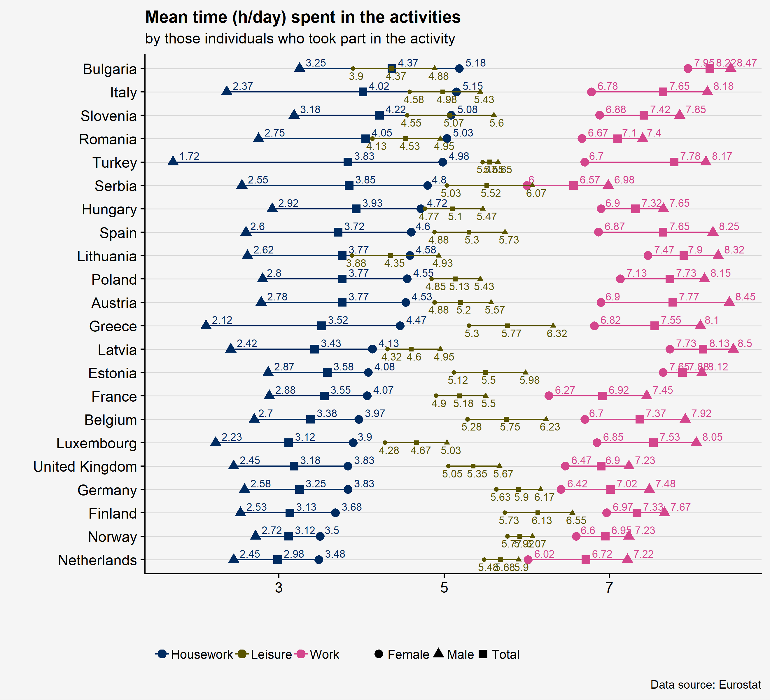
Main observations:
- In all countries women:
- do more housework,
- spend less time in paid work
- have less time for leisure.
- There is a greater gender equality in Scandinavian countries (Netherlands, Norway, Finland)
Comparison in time
dat6 <- dat[nn==6, ]
dat6[, nn:=NULL]- Countries ordered by “Housework”
tmp <- dat6[act=="Housework"&sex=="F"&time=="2010", .(geo, values)]
new_levels <- tmp[order(values), "geo"] %>% unlist

dat6[, geo2:=factor(geo, levels=new_levels)]
dat6[, sex:= sapply(sex, FUN=switch, "F"="Female", "M"="Male", "T"="Total")]
new_levels <- paste0(rep(new_levels, rep(2, length(new_levels))),"_", c(2000, 2010))
dat6[, geo2_time:=factor(paste0(geo, "_", time),
                         levels = new_levels)]
lab1n <- new_levels
lab1n[seq(2, length(new_levels), by=2)] <- lab1n[seq(2, length(new_levels), by=2)] %>% gsub("_",":", .)
lab1n[seq(1, length(new_levels), by=2)] <- lab1n[seq(1, length(new_levels), by=2)] %>% gsub(".*_","", .)
tmp <- dat6[act!="Leisure",]
p <- ggplot(tmp, aes(x=geo2_time, y=values, color=act)) + geom_point(aes(shape=sex), size=3) +
geom_line() +
geom_line(aes(group=interaction( act, sex, geo)), linetype="dashed") +
geom_text(data=tmp, aes(label = round(values, 2), y=values, vjust=-0.3, hjust=-0.3), size=3)+
scale_x_discrete(labels=lab1n)
tmp <- dat6[act=="Leisure",]
p <- p + geom_point(data=tmp, aes(x=geo2_time, y=values, color=act, shape=sex)) +
geom_line(data=tmp, aes(x=geo2_time, y=values, color=act)) +
geom_line(data=tmp, aes(x=geo2_time, y=values, color=act, group=interaction( act, sex, geo)),
linetype="dashed") +
geom_text(data=tmp, aes(label = round(values, 2), y=values, vjust=1.4, hjust=0.3), size=3) +
coord_flip()
vals <- c("#5a5500", "#d4468d", "#002b61")
names(vals) <- c("Leisure", "Work", "Housework")
elr <- element_rect("#F5F5F5", "#F5F5F5")
p <- p + labs(title="Mean time (h/day) spent in the activities",
subtitle="by those individuals who took part in the activity",
caption="Data source: Eurostat", x ="", y = "") +
theme_hc()+
scale_colour_manual(values=vals)+
theme(panel.background = elr,
plot.background = elr,
legend.background = elr,
legend.title=element_blank(),
plot.title = element_text(hjust = 0),
plot.subtitle = element_text(hjust = 0))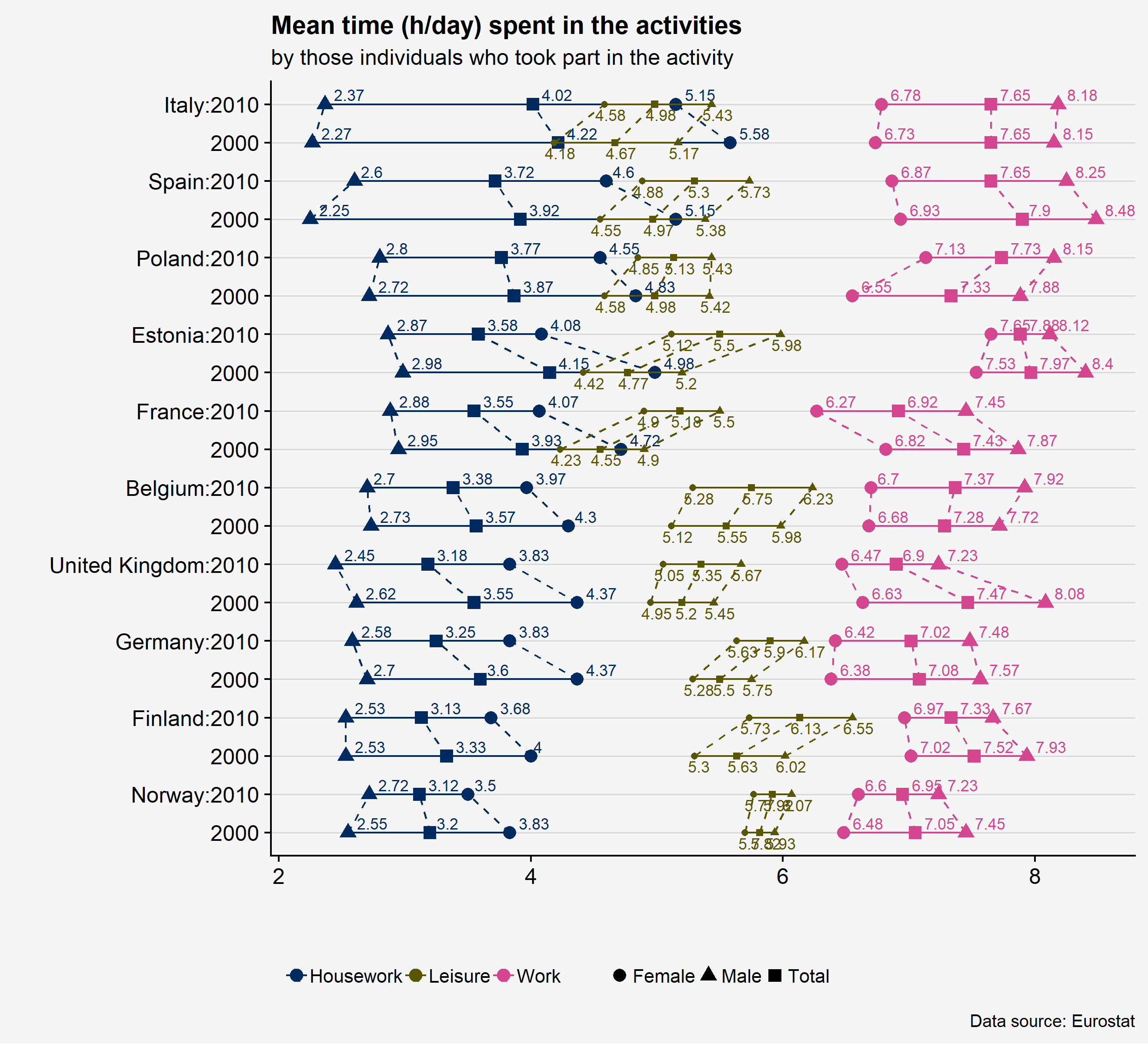
Main observations:
- Gender gap in :
- “Housework” is decreasing (males do more and females less)
- “Leisure” is constant and both genders enjoy more leisure
- “Work” - for some countries work time increased, for some decreased and for some remained almost constant
